How it works: inference jobs

What does a Qualcomm® AI Hub Workbench inference job do?

Inference jobs use real devices in the cloud to run inference on the provided model. The metrics collected are specifically designed to help you determine if a model fits within your time and memory budget, and to collect output data from the provided input data set to help you assess accuracy.

Overview

Qualcomm® AI Hub Workbench runs through these steps to run a Target Model on the specified device:

1. First App Load – The first time a model is loaded, our model runner uses the selected runtime (i.e., Qualcomm AI Runtime, ONNX Runtime, or Lite RT) to load and prepare the model for the hardware. This step may include automatic optimizations for certain hardware, such as neural processing unit (NPU) optimizations when the Qualcomm Hexagon Tensor Processor (HTP) is available. The result is typically cached to make subsequent loads faster.

2. Subsequent App Load – From the second time onward, model loads may avoid costly device-specific on-device optimization to improve speed.

3. Inference – After the model has been loaded, Workbench performs inference. Inference is run on the model several times in a tight loop. This provides a steady state latency that might be achieved in an actual application.

4. Inference by Layer – Jobs with profiling on execute another pass where per-layer metrics are recorded.

For each step, the following time and memory metrics are collected.

Time

Many steps can only be sensibly executed once. For example, it is often impossible to clear all framework and OS caches after First App Load. Therefore, only inference is measured more than once.

Over the course of many iterations, Qualcomm® AI Hub Workbench measures the clock time required to evaluate the model. The cost includes only the cost of the call to the inference framework and a small amount of overhead.

The inference times measured are a microbenchmark whose purpose is to isolate the model from other noise so that it can be meaningfully optimized as an atomic unit.

Memory

There are many ways to characterize the memory usage of an application. To provide clear and comprehensive memory metrics, Workbench reports ranges, which are more accurate than single-number metrics.

NPU Memory

Workbench only measures the memory footprint of the application process itself. To measure the memory consumed on the Hexagon Tensor Processor (HTP), please enable profiling in your inference job and see the HTP Analysis report that is included in the Runtime Analysis section.

Virtual Memory

Modern operating systems provide a layer of abstraction between a user process and physical memory typically called virtual memory. When a process requests memory, few or no addresses are immediately mapped to physical memory. Instead, the OS performs some internal bookkeeping to note that some range of addresses has been promised and that they are clean.

Memory in the clean state has not been written to so its contents need not be preserved if the system runs low on memory. When a process writes to memory, it becomes dirty, meaning the OS cannot independently discard its contents without data loss. If a piece of dirty memory has not been accessed for some period, the OS might free the associated physical memory by writing the data to disk (swapping) or compressing the memory, making it smaller, but temporarily unusable. The memory footprint of an app is the sum of non-clean memory: dirty, swapped, and compressed.

Most Unix-like operating systems, including Android and Linux, do not guarantee that virtual memory can be mapped to physical storage. If global usage is high, demand may exceed the available physical memory and on-disk swap. When that occurs, the system will attempt to preserve its stability by terminating memory hungry processes. Windows takes a different approach: when a process allocates virtual memory, the system commits to store its contents in physical memory and/or page files, ensuring that global demand never exceeds system capacity. Since the system will never run out of memory, terminating overcommitted processes is unnecessary.

Heap

The OS has to manage an unimaginably large virtual address space on modern devices. The metadata required to maintain mappings of virtual addresses to arbitrarily small allocations would be prohibitive for the kernel. Therefore, systems have a minimum allocation size, a page, which is typically in the range of 4-16 KB. Of course, programs usually create objects that are much smaller than a single page. To make efficient use of memory, malloc is used to pack multiple program objects into one or more OS pages.

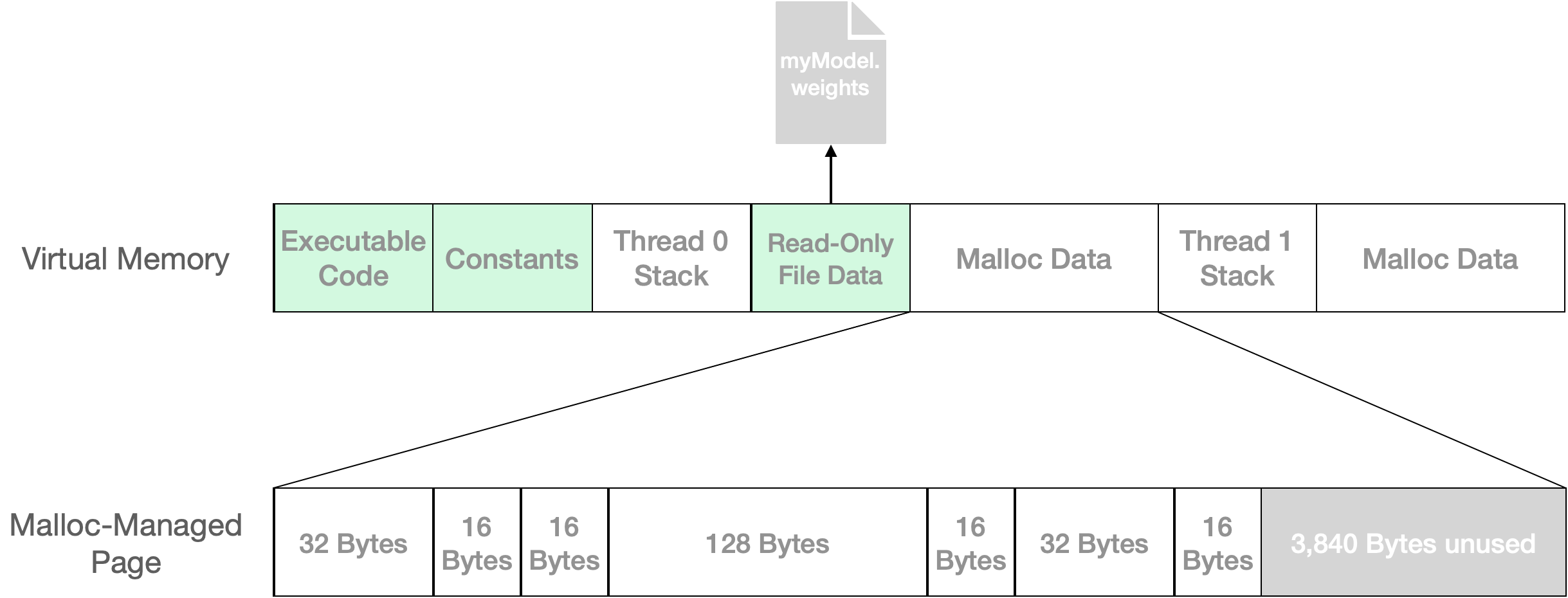
Figure 1: Virtual memory is allocated by the operating systems in units of pages, which may be clean (shown as green) or non-clean. Malloc is an interface to efficiently pack small objects into these large pages. In this example, 256 bytes of user data are packed into a single 4,096 byte page, leaving 3,840 bytes available for future calls to malloc.

Figure 1 shows a simplified virtual memory address space. Clean regions are those that the OS can recreate without running any user code. This is typically because these pages are backed by an unchanging file or simply have not been written to. From some operating systems’ perspectives, non-clean pages constitute an application’s memory footprint: if your app has too many dirty, swapped, and/or compressed pages, it is at risk for termination if the system runs low on memory.

Most runtime data is managed by malloc, whose dirty pages may be only partially utilized. In this example, 256 bytes of user data are held in a 4 KB page, but 3,840 bytes are unused. In real applications, memory hungry tasks such as model compilation and loading can leave considerable amounts of this unused space in malloc-managed pages. This memory can typically be reused by subsequent steps.

In computing a memory footprint, OS-provided tools and APIs are unaware of how much of malloc-managed pages are unused. Since some or all of this unused memory may be reused, on Android and Linux, Workbench reports memory usage as a range that assumes complete reuse in the best case and none in the worst.

As noted above, the situation is different on Windows. Since it is impossible for the system to unexpectedly run out of memory, there is no memory monitor that might terminate a user’s process. Therefore, on Windows, Workbench’s memory usage metrics assume that no already-allocated heap space will be reused by subsequent demands. Both ends of the reported range are the process commit charge, which is the sum of virtual memory allocations. Additional metrics including working set size can be found in the runtime log file.

Peak vs Increase

The memory used to complete a task typically exceeds the size of the result. Consider a scenario where we are compiling a model; assuming no memory leaks in the compiler, it will take some amount of memory to translate an on-device model to a compiled model, leaving an artifact on disk and no objects in memory. If the compiler took 40 MB, we would say that its peak usage was 40 MB, but the steady state increase of memory usage was 0 bytes.

Specific Memory Metrics

Putting it all together, an inference job will return memory metrics like those shown in Table 1. The upper bound of the increase reports a worst-case scenario. Similarly, the amount of data held by the app after loading the model likely does not actually differ between first and subsequent loads, though the initial load left more unused malloc-managed memory. This is not unexpected since the initial load likely did more work and therefore more allocations.

Note that when using offline prepared models for the HTP, such as with a QNN Context Binary, the First App Load will not differ from Subsequent App Loads, because the model is already prepared for the device.

Table 1: Memory metrics for a large CNN model.

Stage	Peak
First App Load	44 - 55 MB
Subsequent App Load	1 - 34 MB
Inference	0 - 32 MB

In Qualcomm® AI Hub Workbench, we present the peak range, which highlights the most important contributions your model makes to memory pressure, which may cause the OS to terminate your app. Those and all other metrics are available in the Python client library (see download_profile). The complete set of memory and timing metrics is shown in Table 2.

Table 2: Metrics returned in the execution_summary of the result of InferenceJob.download_profile.

Key	Type	Units
first_load_memory_increase_range	(int, int)	Bytes
first_load_memory_peak_range	(int, int)	Bytes
warm_load_memory_increase_range	(int, int)	Bytes
warm_load_memory_peak_range	(int, int)	Bytes
inference_memory_increase_range	(int, int)	Bytes
inference_memory_peak_range	(int, int)	Bytes
first_load_time	int	Microseconds
warm_load_time	int	Microseconds
estimated_inference_time	int	Microseconds

Reproducing Metrics

To reproduce the same metrics on your own device, ensure that you configure the runtime with the same configuration parameters as displayed in the “Runtime Configuration” section of the Inference Job details page.

A special note for Android users: the Android operating system schedules foreground UI applications (apps) with a higher priority than CLI applications. This means that tools like qnn-net-run will run more slowly by default than Workbench’s on-device profiler which runs as a foreground GUI app. To have comparable metrics, use a tool like nice to set the priority of your CLI tool appropriately. Note this will only work if you have root access to the device.